Decomposition

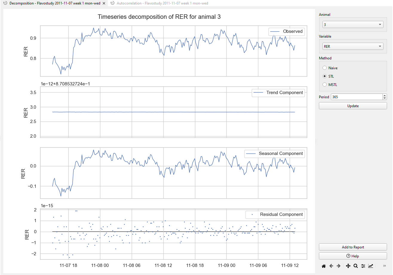
Time series decomposition is a technique used to break down a time series into its constituent components to better understand its underlying patterns, making it easier to model and forecast future values.

The main components of a time series are:

• Observed: This represents the original time series data, showing the unprocessed and complete dataset.
• Trend Component: The trend component displays the long-term movement of the data. It reveals whether the data is gradually increasing, decreasing, or remaining stable over time.
• Seasonal Component: The seasonal component reflects periodic fluctuations in the data, typically occurring at fixed intervals.
• Residual Component: The random noise or irregular component that cannot be explained by the trend, seasonality, or cyclic components. It represents the unpredictable variations in the data.

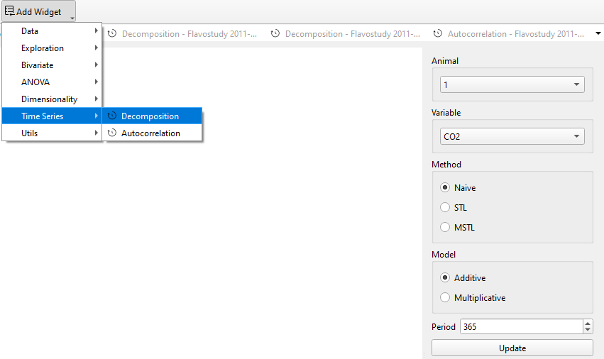
One of three different Methods can be selected: Naive, STL (Seasonal and Trend decomposition using Loess) and MSTL (Multiple Seasonal and Trend decomposition using Loess).

If decomposition is performed using the Naive method, two different models can be used: an additive model or a multiplicative model:

• Additive Model: Assumes that the components add together linearly. Y(t) = T(t) + S(t) + R(t) where Y(t) is the observed value, T(t) is the trend component, S(t) is the seasonal component, and R(t) is the residual component.
• Multiplicative Model: Assumes that the components multiply together. Y(t) = T(t) * S(t) * R(t)

The number of time bins defining the (expected) period of the seasonality, i.e. length of one time cycle, can be set under Period. Setting an appropriate period helps the software accurately detect repeating patterns and seasonal trends in the data.