Variables
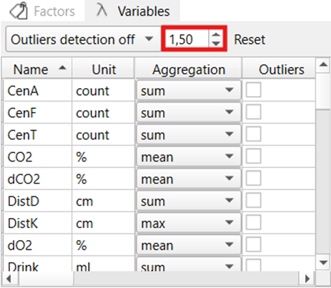
The Variables Widgets in TSE Analytics allows users to select and manage experimental variables. Users can configure aggregation methods for each variable, such as mean, sum, or other statistics. Selected variables are automatically applied to downstream components, including Matrix and PCA statistical tools, ensuring analyses use a consistent and properly processed dataset.
The Variables interface also allows users to delete a selected variables by clicking the delete button or add custom variables by clicking the Add button.
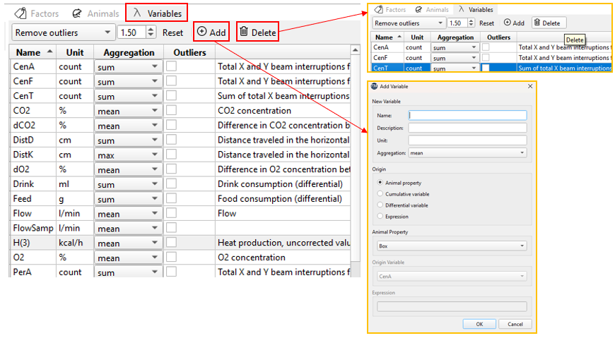
Similarly to Animals widget, in order to select all variables at once, please press
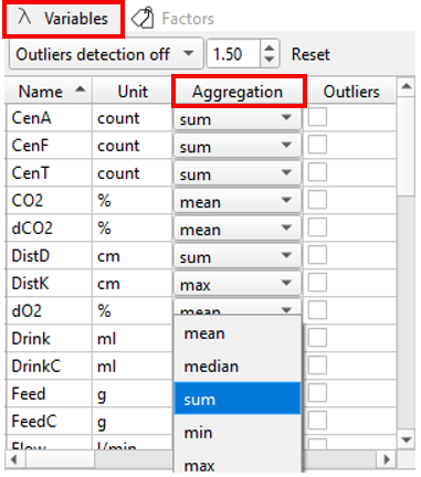
Aggregation
Different methods of calculation (Aggregation modes) can be used for the calculation of data values for individual time bins during binning(i.e., when raw data are grouped into defined time intervals): mean, median, sum, minimum and maximum.
The Binning widget and its settings will be described in detail in the following section.
Note
For cumulative variables, such as DistK,the default aggregation mode is max. Within each time bin, this mode reports the maximum cumulative value, corresponding to the total distance reached by the end of that interval.
If you are interested in the distance covered within each interval (i.e., interval-based activity), you can use the differential variable DistD and apply aggregation modes such as sum or mean.
The default aggregation mode is only a suggestion; users can adjust it according to specific analysis needs.
These modes can be specified individually for each variable via the dropdown menu in the Aggregation column of the Variables widget. The most suitable aggregation mode differs between variables depending on the way data is collected and displayed during a PhenoMaster experiment.
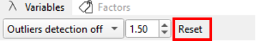
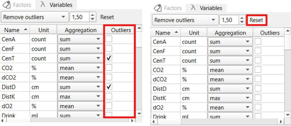
The default aggregation mode is the recommended method of calculation. Aggregation modes for all variables can be reset to the default state by clicking Reset in the header of the Variables widget.
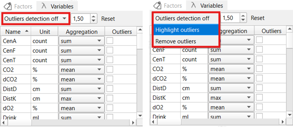
Outlier Detection
Outlier detection settings can be adjusted in the Variables widget. Here, one can choose between different modes via the dropdown menu: no outlier detection (Outliers detection off), highlighting outliers in the data table (Highlight outliers), and removing outliers from the dataset (Remove outliers).
The sensitivity of outlier detection can be adjusted via the coefficient (for further information about the outlier detection method used (please see below: IQR method for outlier detection). Decreasing the coefficient will result in more values being identified as outliers, while increasing the coefficient will result in less outliers.
The variables to which outlier detection should be applied, need to be selected using the tick boxes in the ‘Outliers’ column in the Variables widget. Only variables selected here will be considered for the identification of outliers. The variable selection for outlier detection can be reset to the default (no variables selected) together with the aggregation mode selector by clicking Reset in the Variables widget.
Warning
Selecting Remove outliers will not only delete outlier values but the whole row (i.e. time bin) in the data set which contains one or more values detected as outliers. This means that values of all variables recorded at the same time point as the outlier are removed from the dataset as well.
Therefore, it is recommended to only select the variable(s) for outlier detection which are used for subsequent analysis.
IQR method for outlier detection
- In TSE Analytics, the Interquartile Range (IQR) method is used to detect outliers. This approach identifies outliers by examining the middle 50% of the data.
- The dataset is first sorted, and three quartiles are calculated: the first quartile (Q1, 25% of the data ≤ Q1), the second quartile (Q2, the median), and the third quartile (Q3, 75% of the data ≤ Q3). The IQR is defined as IQR = Q3 − Q1, representing the range of the central half of the data. A coefficient k (default is 1.5 in TSE Analytics) is then applied to define the bounds: Lower Bound = Q1 – k × IQR, Upper Bound = Q3 + k × IQR.
- All data points outside of the range [Q1 – k × IQR; Q3 + k × IQR] are considered outliers.